Sparklines in Microsoft Excel to Visualize Data Quickly

Sparklines in Microsoft Excel Traiing

In Microsoft Excel, some of the new features introduced in the past 15 years are amazing for every day use. Spark lines and Slicers are some of these amazing gems of Excel.

These improvements to PivotTables and other existing features, can help us to discover patterns or trends in the data. To get started with the features of Excel, first we will look at the details of the  Sparkline and slicers features of Excel.

What are Spark lines in Excel, and How to Use Them

Sparkline in Excel
Sparkline in Excel

Sparklines are tiny charts that is used to fit in a cell to visually summarize trends beside the data. 

Sparklines are an extremely useful and user friendly feature in Microsoft Excel that allow you to create small, visual representations of data trends within individual cells.

These tiny charts provide a compact way to display trends, variations, and patterns in your data without taking up a lot of space. Sparklines are particularly useful when you want to quickly analyze data at a glance or within a confined area, such as a cell or a small column.

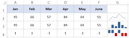
There are three main types of sparklines in Excel:

  1. Line Sparklines: Line sparklines show trends over a period of time. They are typically used to display data points in a line chart format, helping you visualize trends, fluctuations, and patterns over time.
  2. Column Sparklines: Column sparklines are used to compare values among different data points. They can help you identify variations and relative sizes of data within a specific context.
  3. Win/Loss Sparklines: Win/loss sparklines are used to represent binary data, often indicating “win” or “loss” scenarios. These are typically shown using icons or symbols to denote positive or negative outcomes.

Since sparklines show trends occupies less space, they are exclusively useful for dashboards and other places where we need to show a glimpse of the business in an simple practical visual format.

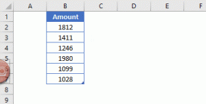
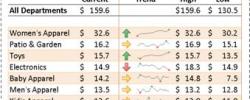
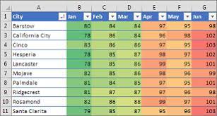
In the image to the left, the sparklines that appear in the Trend column lets us have a quick look of the performance of each department in the month of May.

If you want to join our Excel course in Singapore & improve your skills, we have multiple courses – Basic Excel for Analytics, Advanced Excel Courses in Singapore & VBA Macro Programming Courses.

Key features and benefits of Spark Lines in Excel include:

  • Compact Representation: Sparklines are designed to fit within individual cells, making them an efficient way to provide data insights in a constrained space.
  • Visual Analysis: By using simple visual cues, sparklines allow you to quickly identify trends and patterns, even without delving into detailed data analysis.
  • Easy to Create: Creating sparklines in Excel is straightforward. You can insert sparklines through the “Sparkline Tools” tab on the Excel ribbon after selecting the data range you want to visualize.
  • Dynamic Updates: Sparklines are dynamic, meaning they update automatically when you change the data or adjust the range they’re based on.
  • Conditional Formatting: You can apply conditional formatting to sparklines, enhancing their visual impact. For example, you can color-code sparklines based on specific conditions, making trends more apparent.
  • Compatibility: Sparklines are available in most modern versions of Excel, including Excel 2010 and later.

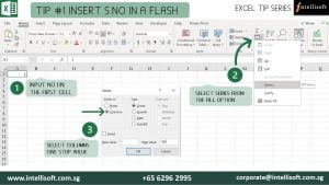
To Create Spark lines in Excel:

  1. Select the cell where you want the sparkline to appear.
  2. Go to the “Insert” tab on the Excel ribbon.
  3. In the “Sparklines” group, choose the type of sparkline you want (Line, Column, or Win/Loss).
  4. Select the data range you want to visualize.
  5. Click “OK,” and the sparkline will be generated within the selected cell.

Remember that while sparklines provide a quick and visual overview of data trends, they might not replace the depth of analysis that larger charts or graphs can offer. Use sparklines in scenarios where space is limited and you need to provide a concise snapshot of data trends.

When and where is the best use of Excel sparklines

Excel sparklines are best used in situations where you need to provide a quick and concise visual representation of data trends within a limited space.
They are particularly effective when you want to highlight trends, variations, and patterns in your data without the need for extensive data analysis. Here are some scenarios where Excel sparklines can be most beneficial:
  1. Dashboards and Reports: Sparklines are ideal for creating dashboards and reports that require a compact presentation of key performance indicators (KPIs) and trends. You can include multiple sparklines in a small area to provide an overview of various metrics.
  2. Tables and Data Lists: When working with data tables or lists, you can add sparklines next to numeric data to provide context and visual insight into how values are changing over time or between categories.
  3. Financial Data: Use sparklines to visualize changes in financial data, such as stock prices, revenue, expenses, or budget allocations. Line sparklines can help show trends over time, while column sparklines can highlight variations between categories.
  4. Project Management: Incorporate sparklines in project management to illustrate task completion, project progress, or resource allocation. For instance, you can display task completion rates using win/loss sparklines.
  5. Sales and Marketing: Use sparklines to represent sales figures, conversion rates, or website traffic data. These visualizations can help sales and marketing teams quickly assess performance.
  6. Comparative Analysis: When comparing data sets or categories, column sparklines can show relative values and trends, making it easy to identify patterns and outliers.
  7. Scorecards: In performance scorecards or performance reviews, sparklines can visually summarize an individual’s progress or achievement over time.
  8. Educational Purposes: Sparklines can be used in educational materials to help students understand data trends and patterns, making learning about data analysis more engaging.
  9. Emails and Presentations: Incorporate sparklines in emails or presentations to provide a quick visual representation of data trends without overwhelming the audience with extensive charts.
  10. Data Visualization in Cells: In spreadsheets where you need to keep the data and visualizations together, sparklines offer a convenient way to incorporate visual insights directly into the data cells.

While sparklines are excellent for providing quick insights, they might not replace the need for more detailed charts and graphs in situations where deeper analysis is required.

Additionally, when using sparklines, it’s essential to ensure that the data you’re visualizing is appropriate for the type of sparkline you’re using (line, column, or win/loss) to ensure accurate representation.

What are Slicers in Microsoft Excel

Excel Slicers Sample

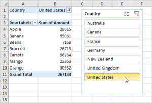
Slicers are visual controls. They let us quickly refine data in a PivotTable in an interactive, automatic manner. If we insert a slicer, we can use buttons to quickly segment and refine the data to display appropriate results.

Not only that, when we apply more than one filter to the PivotTable, we no longer have to open a list to see which filters are enforced to the data. Rather, it is displayed on the screen in the slicer.

We can make slicers relate to the workbook formatting and easily reuse them in other PivotTables & PivotCharts.

Slicers provide an intuitive and user-friendly way to filter and analyze data without the need to access complex filter menus or dialogs.

Slicers create buttons or visual elements that you can click or select to filter data, making data analysis more dynamic and accessible.

When you insert a slicer into an Excel workbook, it creates a dashboard-like interface where users can easily filter data by clicking on specific elements. Slicers are especially useful for large datasets and complex reports where traditional filtering methods might be cumbersome.

When to Use Slicers in Excel:

  1. Pivot Tables and Pivot Charts: Slicers are primarily designed to work with pivot tables and pivot charts. They enhance the usability of these tools by providing a simple way to filter and slice data dynamically.
  2. Large Datasets: When dealing with large datasets, using traditional filter dropdowns can be overwhelming. Slicers offer a more user-friendly experience by visually representing filtering options.
  3. Interactive Dashboards: If you’re creating interactive dashboards or reports, slicers can be a great addition. Users can quickly filter data to focus on specific aspects of the report.
  4. Data Exploration: When you want to explore data trends and patterns quickly, slicers allow you to filter data on the fly without the need to constantly modify filter settings.
  5. Collaborative Work: Slicers are particularly useful in collaborative environments where multiple users need to analyze data. They provide a consistent and easy-to-understand filtering interface.
  6. Sales and Marketing Analysis: Slicers are beneficial for sales and marketing reports where you want to analyze data by different criteria such as time periods, regions, products, or customer segments.
  7. Comparative Analysis: Slicers can be used to compare data across different categories, allowing you to instantly switch between various data subsets for comparison.
  8. Data Visualization: When creating presentations or reports for non-Excel users, slicers provide a more intuitive way to interact with and explore data.

How to Use Slicers in Excel:

  1. Create a Pivot Table or Pivot Chart: Before adding slicers, you need to create a pivot table or pivot chart based on your data.
  2. Insert Slicer: Go to the “PivotTable Analyze” or “Analyzing” tab on the Excel ribbon, then click on the “Insert Slicer” button. Choose the fields you want to use as slicers.
  3. Arrange Slicers: Once inserted, arrange the slicers on your worksheet as needed. You can resize them, move them around, and align them to create an organized layout.
  4. Filter Data: When you interact with a slicer by clicking on an element (e.g., selecting a specific category or time period), the associated pivot table or pivot chart will instantly update to show the filtered data.
  5. Multiple Slicers: You can insert multiple slicers based on different fields to provide more comprehensive filtering options.

Remember that while slicers are a fantastic tool for interactivity and data analysis, they are best suited for scenarios involving pivot tables and pivot charts. For traditional data tables, you might want to stick with standard filtering options.

excel trainingIf you would like to learn more about these new features of Microsoft Excel, or would like to attend the Advanced Microsoft Excel Training, do contact us at Intellisoft Systems.

If you have any further questions or want to join a training on how to use Sparklines, contact Intellisoft for Corporate Training on Excel or call at +65 6250-3575.

Trainer: We have certified trainers who excel in imparting their knowledge and are very patient. Master Trainer Vinai teaches Advanced Excel Techniques, Dashboard Techniques using Excel,  Advanced Data Analytics & Data Visualization Training courses at Intellisoft.

Vinai has trained over 15,000 students in over 18 countries, and regularly conducts Excel Workshops in Singapore, Malaysia, Indonesia, Australia, India, Dubai, Egypt, Zimbabwe, South Africa etc.

Conditional Formatting in Microsoft Excel For Better Data Visualization

Conditional Formatting in Excel using Color Scales for Data Visualization Training

Improved conditional formatting in Excel For Better Data Visualization

Conditional Formatting in Excel - Sample Screenshot
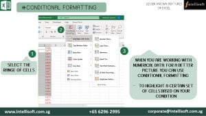
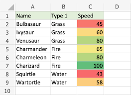
Conditional formatting makes it easy to emphasize important cells or ranges of cells, highlight unusual values, and visualize data by using data bars, color scales, and icon sets. In each newer version of Excel, it includes further more formatting flexibility.

Conditional formatting in Excel is a powerful feature that allows you to automatically apply formatting to cells based on specific conditions.

It’s a fantastic tool for visualizing data trends, highlighting important information, and making your spreadsheets more informative and user-friendly.

If you want to join our Excel course in Singapore & improve your skills, we have multiple courses – Basic Excel for Analytics, Advanced Excel Courses in Singapore & VBA Macro Programming Courses.

Here are some of the best ways to use conditional formatting, along with concrete examples:

Color Scales in Excel Conditional Formatting

  1. Color Scale for Data Ranges:
    • Use a color scale to visually represent the distribution of data values within a range.
    • Example: Apply a green-to-red color scale to a list of temperature readings to quickly identify hot and cold temperatures.
  2. Icon Sets for Comparisons:
    • Apply icon sets to cells to compare values and show trends using icons like arrows or traffic lights.
    • Example: Use upward and downward arrows to indicate whether sales figures have increased or decreased compared to the previous month.
  3. Data Bars for Proportional Data:
    • Use data bars to create horizontal bars within cells to represent the proportional value of each cell compared to others.
    • Example: Apply data bars to visualize the relative sizes of monthly expenses in a budget spreadsheet.
  4. Highlighting Duplicates and Unique Values:
    • Apply conditional formatting to highlight duplicate or unique values in a range of cells.
    • Example: Highlight duplicate names in a list of customers to identify potential data entry errors.
  5. Color-Coded Prioritization:
    • Use conditional formatting to color-code cells based on priority levels, making it easy to identify important tasks or items.
    • Example: Color-code tasks in a to-do list as high, medium, or low priority.
  6. Custom Formulas for Complex Conditions:
    • Create custom formulas for more complex conditions that aren’t covered by built-in formatting rules.
    • Example: Apply conditional formatting to highlight cells with values greater than the average of a range.
  7. Highlighting Dates:
    • Apply conditional formatting to highlight dates that fall within a certain range, such as upcoming deadlines or overdue dates.
    • Example: Use red formatting to highlight dates that are past the current date in a project timeline.
  8. Data Validation Feedback:
    • Use conditional formatting to provide feedback on data validation rules, making it clear why certain entries are invalid.
    • Example: Apply a red border to cells that contain text longer than a specified character limit.
  9. Heat Maps for Data Analysis:
    • Create heat maps by applying conditional formatting to visualize patterns and trends in large datasets.
    • Example: Apply color scales to sales data to quickly identify regions with the highest and lowest sales figures.
  10. Formula-Based Alerts:
    • Use conditional formatting to trigger alerts or notifications based on specific formula-driven conditions.
    • Example: Apply a bold font and red text to cells where inventory levels are below a certain threshold.Icons for use in Conditional Formatting of Data in Excel

Key to effective conditional formatting is to choose formatting options that align with your goals and data presentation needs. By using conditional formatting strategically, you can make your data more visually engaging and facilitate better decision-making.

New icon sets: In Excel, we  can access to more icon sets, including triangles, stars, and boxes. We can also mix and match icons from different sets and more easily hide icons.

For example, we might choose to display icons only for high profit values and remove them for middle and lower values.

More options for data bars: Excel now comes with new formatting options for data bars. You can apply solid fills or borders to the data bar, or set the bar direction from right-to-left instead of left-to-right.

Not only that, data bars for negative values appear on the opposite side of an axis from positive values.

excel trainingIf you would like to learn more about these new features of Microsoft Excel for data analysis and data visualization or would like to attend the Microsoft Excel Training, do contact us at Intellisoft Systems.

If you have any further questions then contact us through email training@intellisoft.com.sg or call at +65 6250-3575!!!

The Best Trainer for Advanced Data Analytics With Excel in Singapore

Mr. Vinai, Prakash the founder of Intellisoft Systems teaches Advanced Excel Techniques, Dashboard Techniques using Excel, Data Interpretation and Analysis Training courses at Intellisoft.

He has trained over 15,000 students in over 18 countries, and regularly conducts Excel Workshops in Singapore, Malaysia, Indonesia, Australia, India, Dubai, Egypt, Zimbabwe, South Africa etc.

Learn Excel Lookup Functions Easily

Some of the most popular Excel Lookup reference functions are VLOOKUP & HLOOKUP.

A newly added XLOOKUP is becoming very popular too. (XLOOKUP is currently only available in Office 365 versions). At Intellisoft, you can learn it by joining the XLOOKUP Training course in Singapore using Microsoft Office 365.

For the power users of Excel, the mastery of INDEX, MATCH & OFFSET can be considered vital, as these are considered the advanced lookup functions in Excel.

These functions will help you Analyze Data quickly. You should enrol in the data analysis and interpretation training class in Singapore.

But with the introduction of XLOOKUP, some of the jugglery created by mixing INDEX & MATCH combination is no longer required.

VLOOKUP Function of Excel

The most MUST HAVE Function ever. Even Excel gurus can’t live without it. I polled a group of Excel experts recently, asking if Excel’s VLOOKUP was overrated. I got a severe backlash for even mentioning it.

Almost everyone said that it is their GO TO function, an absolute must-have and that Excel won’t be that useable if this VLOOKUP function was taken away from Excel!

Most people swear by their VLOOKUP functions. It is their GO TO function when they want to lookup value of any type.

According to legend, VLOOKUP mastery is what separates the Pro Excel users from the Amateurs!

Vlookup is akin to using a dictionary. You know the word, and you want to find out the meaning. This dictionary is the range of cells that contain the lookup up value, and its associated value. The V in VLOOKUP stands for the dictionary being a vertical dictionary. So for a vertical lookup, you must use VLOOKUP function only.

=VLOOKUP(word, dictionary, column number of meaning, exact_match_ype)

The first column in the dictionary must contain the lookup up value, and the first row should be of the data. You should not include the headings in the dictionary table. The difficulty most people have with VLOOKUP is the last flag – the logical value of TRUE or FALSE (You can use 1 for True and 0 to indicate the False flag).

Once a matching value is found out, you will be able to get the return value based on the search. The error value of N/A will be generated if there is no exact match until the last row.

The mystery is created because to use VLOOKUP for an exact match, you have to specify the last optional flag, and set its value to a FALSE or a 0. By default, it is set to 1, which is useful for an approximate match type only. So for an exact match of a specific value, the last parameter is not really optional… it is mandatory.

VLOOKUP EXAMPLE:

There are a couple of major shortcomings in using VLookup function of Excel. First of all, the VLOOKUP is really a slow function. It is apparent when you do a lookup on a large list of 100,000 values or more. Secondly, VLOOKUP can only look up up a corresponding value from the columns on the right of the looked-up value. It can’t look to the left!

Make sure you master this Excel function really well.

HLOOKUP Function in Excel

An oft-forgotten cousin of VLOOKUP, this Horizontal Lookup and Reference function in Excel works in a similar way too. The only difference is that in this case, a lookup dictionary is a horizontal dictionary of columns, denoted by the H.

HLOOKUP is most used in range lookups, rather than exact matches, as columns are not the best suited for exact values, because of their limit of 16,000. Where a list can grow vertically to over a million records easily.

In the following formula, this lookup function searches for the closest match, especially when we are not searching for an exact match, but an approximate match. The dictionary is the table array and it is recommended that we use the absolute reference to lock the cells from moving.

=HLOOKUP(A5, $G$2:$K$100, 2)

Here the HLOOKUP will search for the exact or the next smallest value in the lookup table absolute range of $G$2 to $K$100, and return the second row. If you want the third row, you can change the 2 into a 3.

Both VLOOKUP & HLOOKUP return values from a single row or a single column.

Using the XLOOKUP Function in Excel

Did you know that new functions are added to Excel till today, and these are extremely useful functions making approximate matches as well as exact matches.

Finally, after years of backlash at Microsoft for creating the mess with the Match Type (True and False) in VLOOKUP, they got rid of it completely in the Excel XLOOKUP function.

And by default, XLOOKUP is set to do an exact match.

XLOOKUP requires a deeper understanding of the various scenarios. I’d recommend attending our formal ADvanced Excel Training to build a strong foundation in Excel. You can call us at 6250-3575 for more information of our courses and available enrollment dates for classroom training in Singapore.

This new XLOOKUP function of Excel is only available from Microsoft Office 365 users. It does not work on Excel 2016 or Excel 2019 versions.

Using INDEX Function in Excel

If you know the row number, you can find the value on that row or column cell directly.

INDEX can be used as an Array function also. Paired with MATCH, you can find any value on any row or column in a 2-dimensional array.

Index can help you to find the value on the row or the column of the specified number

How To Use Excel MATCH Function

When you want to find an exact match in an array and return the row number in the array, MATCH comes to your rescue. It is one up on VLOOKUP, which requires you to know the column you want to return. MATCH can find a match for a value that is lower, exactly equal or higher than the specified value.

Paired with INDEX, an INDEX & MATCH Function can manage to look up on the left or the right of any array of cells.

Master the OFFSET Function within Excel

To navigate your way in a two-dimensional array of rows and columns, you can use the OFFSET function in Excel. It can traverse any number of Rows or Columns, and get you the value.

How to use the offset function in Excel:

=OFFSET(Starting Cell, Row to move up or down, Columns to move left or right, Number of rows required to be returned, number of columns required to be returned)

I generally use OFFSET more than INDEX and MATCH combinations. Using one super-powerful OFFSET function is more straightforward.

Once you start using Offset in Excel, you wouldn’t want to use other lookup functions of Excel.

When Do I Use the INDIRECT Function of Excel?

The Excel INDIRECT function returns the reference specified by a text string. References are immediately evaluated to display their contents.

Use the INDIRECT function when you want to change the reference to a cell within a formula, without changing the formula itself.

=INDIRECT(A3)

The above Indirect function will check what is in cell A3. And A3 will have the cell reference to another cell. So if A3 contains B35, Excel will then read the value in cell B35.

Thus, we can get the value of the reference in cell A3. The reference is to cell B3, which may contain the value 45.

The INDIRECT can be very useful in creating custom management dashboards and reports.

What does the FORMULATEXT Function of Excel Do?

Displays the text of another formula. This helps to see all formulas next to their values and can be useful to spot mistakes and issues with formulas.

=FORMULATEXT(A3) will provide you with the formula in cell A3 as a Text Value.

This FormulaText function is useful to see the formula without having to go into Editing mode.

View this link for more information on how to get the Formula of another cell in Excel.

How to use ROWS Function of Excel

Displays the row number of a reference cell.

=ROWS(A1:B4)

Will return a 4. This is because there are 4 Rows in the given range.

How to Use the COLS Function in Microsoft Excel?

Displays the column number of a reference cell.

=COLS(A1:B4)

Will return a 2. This is because there are 2 Columns in the given range: A & B

Using the TRANSPOSE Function of Excel like a Pro

Converts rows into columns and columns into rows. Just like the Transpose feature in Paste Special, but done programmatically.

So if you use TRANSPOSE(A1:D3), you have selected 4 columns and 3 rows.

After the Transpose is completed, you will get an array reference of 3 Columns, and 4 Rows. The horizontal table would have flipped and will be visible vertically.

Pretty nice use of hanging values in rows into columns.

When Do I Use the UNIQUE Function of Excel?

The UNIQUE function of Excel generates a list of unique values that automatically spill down. An array function can be used to create data validation lists too. Available from Microsoft Office 365 onwards. This UNIQUE function is not available in Excel 2016 or Excel 2019.

Learning the Lookup Functions in Excel Quickly & Easily

As you can see, there are a lot of LOOKUP functions in Excel, and learning and mastering them takes time. But once you do master them, you can do wonders with your Excel skills.

It is worth the effort to learn the Excel Lookup Functions. Call Intellisoft at 6250-3575 or What’s App at +65 9066 9991 for Excel 365 Training that covers the key Lookup functions of Excel.

You will definitely enjoy it!

Cheers,

Vinai

Founder & Master Trainer at Intellisoft Systems in Singapore.

Are You Microsoft Office Proficient?

Microsoft Office Training in Singapore

Every job seeker would have this word written in their resume Microsoft Office Proficiency.  

What Exactly is Microsoft Office Proficiency?

A Microsoft Office Proficient should be able to create an error-free, beautifully formatted document with header, footer, page number & Page breaks.

In Excel, they should be able to handle a large volume of data, format, sort, filter and create Pivot Tables for better visualization of Data.

In PowerPoint, the ability to make aesthetically appealing stellar presentation with graphics, images, GIFs, Animation is considered good proficiency.

Handling Microsoft Outlook like a pro to manage emails, create separate folders, track tasks, manage calendar, set reminder, marking them complete, and most important, getting things done quickly with these productivity tools.

This should not be overwhelming. It should be easy to do, and management expects everyone to be proficient in Microsoft Office.

It has been years since the Microsoft Skills have become mandatory for every person coming into the workforce – whether administration, data handling, HR or even the Managerial Position.

A research by IDC concludes that Microsoft Office is one of the top three skills desired by any employers next to oral and written communication Skills.

Possessing Microsoft Skills not only merely helpful in typing docs and tabulating number, rather they help us to get more productive, efficient and handle and present data professionally effectively than ever. Microsoft Office is the most effective, accessible, and easy to use software’s.

Lear Microsoft Office Skills at Intellisoft

Microsoft Word:

It has been used by many people as just a notepad or a typing software’s. But in real, it can do wonders in creating professional Documents.

If we can spend some time in learning a bit more than what the Home Tab has, it can considerably reduce the time we spend on making documents.

Word is useful to create better Proposals, Reports, Agenda, Meeting Minutes & more.

Microsoft Excel:

Excel is often used in accounting and finance for its ability to calculate and compute complex numbers. Even non-financial businesses use Excel because of its unbeatable ability to organize data in tables & for updating, organizing, and displaying the data nicely.

It is highly used in administration and managerial level to analyze data quickly and present to management.

It even supports Visual Basic Applications to create macros to automate functions that increase efficiency.

In fact, the Pivot Tables and Dashboards are inevitable when it comes to analysis and reporting. You must up your proficiency in Excel to master these functions.

Microsoft PowerPoint:

Everyone would have made a basic presentation in Schools and workplaces to present the work. But PowerPoint comes handy to make it visually appealing and effective.

Its intelligence in generating different design ideas for the slides is becoming so popular nowadays. Other than just suggestion, it allows you to use the plenty of shapes and icons that are in-built and even allows you to import illustrations and graphics from the internet while working.

In short, anyone can make a stellar presentation with a quick guidance and practice.

It is always wise to have a most sough after skill in hand to increase employability & cement a position in job industry.

While Microsoft Office is filled with short cuts and methods to create attractive and easy to manage documents, a comprehensive hands-on training can help you to master the hooks and corners of the Microsoft Office package within just 3 days.

Simply follow the step-by-step instructions and learn the art of creating professional business documents easily every time.

With this training you will be able to Create Impressive Proposals, Charts & Presentations to Woo Clients.

View the detailed Course Outline

Companies can apply for SDF FUNDING & Individuals can apply for SkillsFuture Credits to offset the Training Fees.

If you have questions on Funding or need an official quotation/course brochure, please contact me on 9343-2080 or drop us an Email.

Like us on Facebook, Follow us on Instagram and Do Check out our LinkedIn for more updates on the Courses & Grants!

P.S: Don’t forget to check out our Amazing Article on Best Practices For Managing Emails With Microsoft Outlook to Manage Emails like a Pro!

Exciting Microsoft Excel Shortcuts You Never Knew

Top-Exciting-Microsoft-Excel-Shortcuts-You-Never-Knew

Microsoft Excel is one of the most used software at work. People who claim to know Microsoft Excel software mostly are the ones with basic or intermediate knowledge & understanding of Excel. The productivity increases only when we make the most out of the useful software, and gain mastery.

There are many hidden gems and short cuts within Excel, that hardly anyone talks about. I am amazed when people with years of Excel experience tell me they haven’t heard about these. What a waste of time…

‘Let us discuss in this series the ultimate tips in Excel that will make things snappier, and make your co-workers say, “how did you do that??”. They will save a lot of time for you too and improve your productivity.

Tip Number 01 INSERT SERIAL NUMBERS IN A FLASH

What do we when we have to insert Serial Numbers in Excel? We type the number 1 in the cell A1, then 2 in the cell A2, and finally select both the cells & drag the mouse pointer until we get the required serial numbers generated. Right?

But what happens when we need Serial numbers until 100? 200? Or more?

Do we keep dragging? Certainly not!

There is an ultimately easy way in which you can just flash fill the serial numbers to whatever value needed.

Insert Serial Number in a Flash

Here are the steps:

Input Number 1 in the first cell

Step 1 Input number in Cell A1

Select Fill > Series from Editing Ribbon of Home Tab

  1. Home> Fill > Series

Step 02 Select Series from Fill option

  • Select Columns from the Dialog box, give Step & Stop values and Hit OK.

Step 03 Select Column and give stop value

NOTE: If you are looking to Fill Rows instead of columns, just select Rows in the dialog box and follow the same steps.
Bet you didn’t know this trick… Well, now you do.

Tip Number 2 FORGET COPY+PASTE – JUST DRAG & DROP

When we have a set of data in one column & we want it to move to another column. What do we do? Select them all, copy or Hit CTRL C and select the destination column, and paste or hit CTRL V?

Forget the hassle, now select the required data, just Drag & drop to the destination.

Drag and Drop to Copy

Tip Number 3: COPY MULTIPLE VALUES USING THE CLIPBOARD

Working with multiple values? Forget the hassle of copying and pasting one by one.
Use the built in Clipboard feature of Excel.

You can expand the clipboard from the icon lists or use the Win (Windows Key) + V to click on the required values

Copy Multiple values using Clipboard

Tip Number 4: DUPLICATE A SHEET IN JUST ONE-CLICK

Want to copy the whole sheet? Are you selecting and copy pasting?
Or right click, copy, select the sheet, move to bottom?? So many steps for duplicating the sheet?

Now Duplicate a Sheet like a Pro!

Just hold down Ctrl + Drag & Drop the sheet to desired position.

Duplicate sheet by drag and drop

Tip Number 5: UNDO & REDO IN ONE HIT

Undo & Redo would be the most used operations in Excel.
Now do undo and redo with just one click.
Use the buttons on top.

Undo and redo in one click

Tip Number 6 Use the QUICK ACCESS TOOLBAR

Tedious to find the operations that you frequently use?

CHANGE ALL CAPS TO Mixed Case for Next 3 Rows.

CLICK THE DROP DOWN ARROW TO SEE THE OPTIONS
YOU CAN ADD THE FREQUENTLY USED OPTION TO QUICK ACCESS TOOLBAR

EXTRA TIP: YOU CAN ADD ANY OTHER COMMANDS THAT YOU USE FREQUENTLY

Quick Access Toolbar

Hope that helps! Want to learn more exciting tips, tricks & shortcuts and improve your productivity in Microsoft Excel?

If you wish to build your knowledge to have a better Excel Operations knowledge, you must start working on it. You will do well in your career, and get ahead faster, even land that dream job with better skills & competence in Excel.

We at Intellisoft are here to guide you.

Intellisoft Systems offers 2 day extensive workshops on Microsoft Excel.

Simply pick a program – Basic/Intermediate Excel OR Advanced Microsoft Excel

Join us to get more out of Microsoft Excel to make the best use of the software in your day-to-day work!

Discover Lesser Known Features of Excel

Hidden features of Excel

Want to go beyond the common use of Excel and Explore its Extremely Useful but Lesser-Known Features of Microsoft Excel?

Microsoft Excel’s extensive features can help you to increases productivity and also saves time. Become proficient in Data Management & Business Analytics – Turn Data into Insights, Develop better tables & charts.

Lesser Known Features of Microsoft Excel

Conditional Formatting:

Apply formatting to cells automatically depending on the value of the cell. It is also a powerful feature, given that conditions can be based on any Excel formula. Conditional Formatting works by letting you set rules for how cells can be customized.

Conditional formatting makes it easy to highlight required cells or ranges of cells, emphasizing unusual values. In addition to that, it is used to visualize & analyze data in Excel by using data bars, color scales, and icon sets. Overall, it helps you to identify important data faster.

Learn Lesser Known Shortcuts of Excel at Intellisoft Singapore

Advanced Filters:

This Advanced command works differently from the Filter command in several ways. It displays the Advanced Filter dialogue box instead of the Auto Filter menu. You can filter the data in place, or to a different location. You can also specify that you want to see unique items only.

All the duplicates are removed from the filtered list, with Advanced filter. The Data tab contains all the features of Advanced Filters. The advantage of using advanced filter is that you can see the filtered criteria in Excel cells. You can also easily add new filters by typing the values directly in the cells. Thus, it is absolute must learn feature.

Learn Advanced Filter for more Productivity at Intellisoft Singapore

Database Functions:

Database functions is a Seldom used Gem in Microsoft Excel. With this, you can not only perform basic calculations but also use complex criteria, that allow you to perform the calculation for a specified subset of the records in your database.

These functions treat the entire set as a Database, just like a SQL Database.

Learn the Database Function at Intellisoft Singapore

Consolidating Multiple Worksheet:

If you receive information in multiple sheets or workbooks that you want to summarize, the Consolidate command can help you pull data together onto one sheet. It allows you to combine information from multiple workbooks when you need them one place.

The Excel consolidate function lets you select data from its various locations and creates a table to summarize the information for you, automatically, painlessly.

Learn Consolidate Function at Intellisoft Singapore

Preventing others from Changing Master Data:

This feature allows you to prevent other users from accidentally or deliberately changing, moving, or deleting data in a worksheet. You can lock the cells on your Excel worksheet & then protect the sheet with a password.

With worksheet protection, you can make only certain parts of the sheet editable and users will not be able to modify data in any other region in the sheet.

You can lock the structure of your workbook by specifying a password.
Locking the workbook structure prevents other users from adding, moving, deleting, hiding, and renaming worksheets.

While Microsoft Excel is packed with gems, these are just a few advantages of learning Advanced Excel with us at Intellisoft. We’ll make you an expert in these lesser-known, but advanced features in Excel.

Free Tips, Tutorials & Training Grants Info

Learn from expert tips, tricks and resources for Excel, PowerPoint, Photoshop, Python, Power BI, Project Management, IT, Soft Skills & more with our Email Newsletter.
Plus get the latest news on Grants. Join Today!

Found What You Were
Looking For?

Just Tell us...

We're Here To Help You!